Assignment 5 Report

Exploring potential relationships between S&P 500 firm 10K sentiment and returns post-filing

Summary

The question: Is there a correlation present between positive and negative sentiment exhibited in firm 10Ks and the firm’s stock returns following their filing?

My approach: To determine this, I analyzed data from the firms in the S&P 500 index. I first develop sentiment scores for each based on the words included in their 2021 10-K filings. These scores are based on 10 variables. The first 4 of which are positive and negative literature-based lists from two studies done in the field. The last 6 are positive and negative scores surrounding three topics discussed: Environmental factors, Social factors, and Governance factors. Once the scores were calculated, I then determined the cumulative returns for each firm’s stock from time t (filing date) to t+2, and then again for t+3 through t+10. With these added to the dataset, I was then able to calculate correlation values between the measures of each sentiment score and returns over each of the two periods.

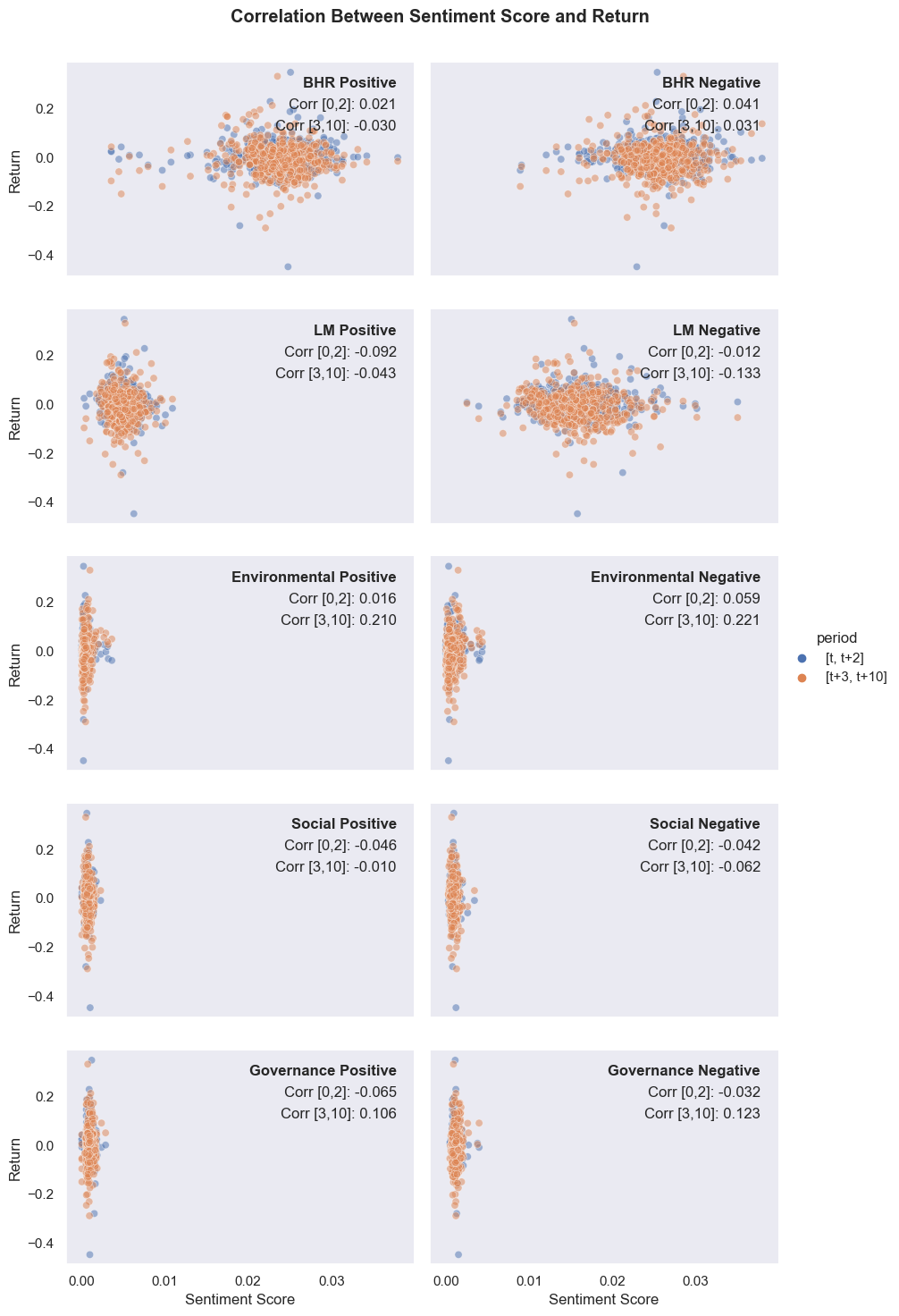
My results: After collecting data on each of the firms, I developed both a table and scatterplot to outline a visualize the various correlations (seen below). Overall, it seems that in the short term following a 10K filing there is a positive correlation for positive BHR words and those surrounding Environmental issues. However, the rest, the correlation is negative over this time period. For the longer-term period returns, for BHR positive, LM negative, and social positive and negative variables, the correlation is negative. For the rest, it is positive.

More discussion on the results can be found below.

Data Overview

Sample:

In this report we look at the firms in the Standard and Poor’s 500 index. As will be described in later sections, certain firms are omitted in different evaluation steps due to factors such as a missing 10K, late report date, and others.

Downloading the 10K Files:

The first step of the analysis was to download the 10K files for the firms in the sample. Using sec-edgar-downloader, the 10K file for each of the firms in the S&P 500 index is downloaded into a folder titled 10k_files. Each document is kept within a parent folder that is named the firm’s ticker. Only the HTML file is saved in order to save space on the user’s computer. Once all of these subfolders are created in the 10k_files folder, the folder is zipped and all empty directories are removed.

Return Variables: The process for calculating the return variables went as follows

Import data on S&P firms
1. Once imported, record firm ticker and CIK values for later analysis
Calculate report date and enter it into the database
1. Iterate through the 10K files downloaded in the previous step that correspond to the tickers in the stock_data database
  1. Reference the CIK already in the database for the firm
  2. Determine the accession number using the 10K filepath for the firm and .split()
  3. Use requests_html with these two values to determine the filing date through the sec.gov website
  4. Add this date to the database for each firm
Import the daily returns
1. Locate the crsp_2022_only.zip file in the course’s data folder
2. Use urlopen and ZipFile packages to read the returns data into a dataframe titled daily_returns
3. Iterate through the firms in the database
  1. Find the index for each [firm, filing date] pair in the daily returns dataframe and save this as index 0
  2. Calculate index 2, index 3, and index 10 by adding to this index number
  3. Determine the cumulative return for days 0-2 for the firm
    1. Find all database entries between calculated index 0 and index 2
    2. Utilize .assign() to apply the daily return for that day
    3. Use .cumprod() to calculate the cumulative return for the firm between t and t+2
  4. Save this [t, t+2] cumulative return to the database
  5. Determine cumulative return for days 3-10 for the firm
    1. Find all database entries between calculated index 3 and index 10
    2. Utilize .assign() to apply the daily return for that day
    3. Use .cumprod() to calculate the cumulative return for the firm between t+3 and t+10
  6. Save this [t+3, t+10] cumulative return to the database

Note: some firms don’t have 10K filings, others have a filing date that is within 10 days of the end of the 2022 year, and some firms filed when they weren’t being traded. All of these firms are omitted from these calculations for the sake of the analysis.

Sentiment Variables: The process for calculating the sentiment scores went as follows

Note: In the initial notes used to import the data the “ML” dataset was titled “BHR”, so that is the value used throughout. I am now realizing the author initials are actually “GHR”, please excuse this.

Create regex expressions for the first 4 of 10 variables (LM positive, LM negative, ML positive (BHR positive), and ML negative (BHR negative)
1. Import positive and negative word lists for BHR and LM utilizing the files in the inputs folder, pd.read_csv(), and .to_list()
2. Cast all LM words to lowercase since they import as entirely uppercase
3. Use ['('+'|'.join(list_name)+')'] to create regex expressions out of each word list
Create regex expressions for three topics: Environmental, Social, and Governance
1. Select the three topics (rationale for choices can be found in the section below)
2. Develop 20 positive and 20 negative words associated with each of the three topics and list them in the form of ['(word1|word2|...|wordN)'] so they can be read by near_regex
In the same for loop as the previous step, iterate through the 10K files that correspond to the S&P 500 firms
1. Use zipfolder to open each 10K
2. Use BeautifulSoup() to open the HTML file of the report and cast all letters to lowercase
3. Remove punctuation to create cleaned string of words
4. Calculate the document word length and add this as a variable in the database
5. Calculate the number of unique words and add this as a variable in the database
6. For each of the 10 sentiment regex expressions developed in the previous two steps, calculate the sentiment score of the document using len(re.findall(NEAR_regex(regex_expression),cleaned_document))/document_length
7. As the scores are calculated, add them to their respective columns in the database

Add additional accounting variables from `2021_ccm_cleaned.dta`

Locate the url for the data file
Use pd.read_stata to open the data as a dataframe
Merge the ccm_cleaned data with the stock_data database using an left merge on ticker (left merge to ensure all variables in the stock_data database are included in the merged dataset

Once this step is complete, we save the merged dataframe as a csv to our output folder.

Rationale for the three topics chosen

When determining the options for the three topics to measure sentiment for, I thought about what is relevant evaluation criteria in the current financial world. The topic of ESG has been at the forefront of most financial discussion over the past few years as the world becomes more cognizant of the damage we are causing the environment, how we should treat others in our communities, and how to best lead a company. As a result, the three topics chosen were:

Environmental: Issues involving how the corporation treats the environment. Takes the form of emissions, waste, energy use, etc.
Social: Looking at how the company interacts with internal and external stakeholders. This includes suppliers, its local community, its employees, workplace culture, etc.
Governance: Looking at, overall, how a company is run. Governance issues would involve how accounting is done, how leadership is decided, if there are conflicts of interest, etc.

Overall, these three areas are ones that are definitely topics discussed in a company’s 10K. Additionally, it is extremely interesting to see if there is a correlation between any of these three factors and a firm’s stock returns after an annual report that addresses them.

Summary statistics of the final analysis sample

An important note to address here is how the count of the firms in the dataset (503) differs from the number of documents read (496), the number of cumulative return calculations (484), and the value counts for the variables merged into the database from the 2021 ccm data. While there are 503 firms in the S&P 500 index, only 496 of them had 10Ks available for download using sec-edgar-downloader. Additionally, of those 496 only 484 of them reported their 10K on a date further than 10 days away from the end of the year. Firms reporting after that point were omitted because there wasn’t 10 days worth of data to calculate a cumulative return on. Lastly, the ccm cleaned dataset is not 100% complete and has varying data for different firms, this leads to some firms listing variable values from the merge and some not.

Second, it is interesting to observe that the average return for the firms over the first 2 days post-report is positive, whereas the average for days 3-10 is negative. This indicates an often initial positive response to the annual report followed by negative sentiment. Another intriguing note is the maximum return values for both [t, t+2] and [t+3, t+10] being over 30%, and the minim return value for the first two days being ~-45%.

Sense-check of contextual sentiment measures

Overall, the sentiment measurements seem realistic when considering the number of words searched for and the length of the document. Since the BHR and LM word lists are longer than those I created for my topics it also makes sense that the sentiment measures for those are greater. There are also no concerning outliers in either the maximum or minimum values of each of the sentiment scores. Judging by the standard deviations, they are all relatively similar. Lastly, there is variation in the data points (they are not all 0 or 1, they all possess varying values).

Data caveats

Some firms omitted for not having a downloadable 10K
Some firms omitted for not reporting their 10K early enough in the 2020 year
Some firms omitted for filing on a date they were not publicly traded
There are some missing values in the ccm data merged with the dataset

The first three caveats address omissions made in the final dataset. The dataframe entries are kept in the sample csv file, but the null values are dropped in the report analysis stage that follows this one. This is due to the fact dropped entries depend on the variable(s) being analyzed. The omissions themselves are to ensure all data points are complete and accurate. For example, if a firm files within 5 days of the end of 2022, the calculation for [t+3, t+10] returns would be inaccurate. Additionally, if a firm doesn’t have a downloadable 10K in the first place or wasn’t publicly traded when the filed, the returns can’t be calculated in the first place.

Results

Correlation table

table = pd.DataFrame()
table['measure'] = analysis_sample.iloc[:,5:15].columns
table = table.set_index('measure')
table['cumret_0-2'] = ''
table['cumret_3-10'] = ''
for row in table.index:
    for column in table.columns:
        corr = analysis_sample[row].corr(analysis_sample[column])
        table.loc[row, column] = corr
table

	cumret_0-2	cumret_3-10
measure
BHR_p	0.021169	-0.030056
BHR_n	0.041228	0.031489
LM_p	-0.09204	-0.04267
LM_n	-0.012259	-0.133046
topic1_p	0.016327	0.209953
topic1_n	0.058547	0.221421
topic2_p	-0.045754	-0.01004
topic2_n	-0.042455	-0.061905
topic3_p	-0.064934	0.10553
topic3_n	-0.03165	0.123202

Scatterplot figure

Note: figure created in exploration_ugly.ipynb and saved to the repo

Discussion

For (1), (2), and (3), the focus is just on the first return variable.

For (4), it is on the ML sentiment variables (positive and negative) and both return measurements.

1. Compare / contrast the relationship between the returns variable and the two “LM Sentiment” variables (positive and negative) with the relationship between the returns variable and the two “ML Sentiment” variables (positive and negative). Focus on the patterns of the signs of the relationships and the magnitudes.

The correlations between the first return variable and the LM sentiment variables are both negative. For the positive side, there is a correlation of -0.092. On the negative side, there is a correlation of -0.012. For the two ML sentiment variables (BHR), both positive and negative sentiments have positive correlations for this return variable (0.0212 and 0.0412 respectively). The signs don’t match here, and neither do the magnitudes. For both BHR and LM sentiment variables the correlations for positive and negative have different magnitudes. This is most likely due to the difference in words in the two datasets.

One thing I found interesting, however, was how the correlation values differed for the second return variable. For time period [t+3, t+10], the positive BHR, was negatively correlated with the returns. It seems that, in the longer term, there is more of a negative return associated with these positive words regardless.

2. If your comparison/contrast conflicts with Table 3 of the Garcia, Hu, and Rohrer paper (ML_JFE.pdf, in the repo), discuss and brainstorm possible reasons why you think the results may differ. If your patterns agree, discuss why you think they bothered to include so many more firms and years and additional controls in their study? (It was more work than we did on this midterm, so why do it to get to the same point?)

Table 3 of the Garcia, Hu, and Roher paper outlines a similar correlation between the BHR/LM sentiment measures and returns. They, however, collect returns over a 4-day period as opposed to our 2-day one. Additionally, it is done over 39,269 observations as opposed to our 484. Garcia, Hu, and Roher analyze all firms listed on NYSE, Nasdaq, and AMEX, that are reported on CRSP as ordinary common equity firms, have 60 days of available trading volume, and have a share price of more than $3 on the day before their earnings call.

My comparison above conflicts with the data shown in this table. My data has positive correlations for a negative sentiment variable (BHR), while the table has a negative one. This is most likely due to the differing time periods used and the varying number of observations. For time period, I also see a negative correlation in days 3-10 for three of four measures, something that more closely aligns with table 2. Additionally, observing returns for stocks in the S&P 500 will certainly be different than data from all firms fitting the criteria mentioned above.

3. Discuss your 3 “contextual” sentiment measures. Do they have a relationship with returns that looks “different enough” from zero to investigate further? If so, make an economic argument for why sentiment in that context can be value relevant.

My three contextual sentiment measures were interesting because of how unexpected their results were. When choosing the ESG factors as my topics, I expected there to be a positive correlation for the positive words and a negative one for the negative one. This was not what I observed. In fact, positive sentiment for both Social and Governance factors was negatively correlated with returns over the [t, t+2] time period. The same was true for the negative versions of those measurements.

One measure that should certainly be looked into further is the positive sentiment for the Governance factor of ESG. The correlation found here was ~-0.06, a measure of one of the largest magnitudes for this time period. What then made it more interesting is the greater-magnitude positive correlation seen in the second returns variable. In the short term, a positive mention of governance principles may be treated as a solution to some problem, causing investors to actually lose confidence in the firm. Over the longer term, however, it seems this corrects after the initial scare subsides and investors grow confident in the corporate leadership once more.

4. Is there a difference in the sign and magnitude? Speculate on why or why not.

There is an observable difference in sign and magnitude between correlations. For the short-term return, the correlation for both positive and negative values is positive. For the return on days 3-10, it is negative for one and positive for the other. Additionally, the magnitude of the positive sentiment correlation is greater in the short term, but magnitude of the negative sentiment is greater in both periods. This is most likely due to the fact that negative sentiment is reacted on more intensely after a report is filed.